Gerrymandering and the Courts According to reporter Adam
Liptak: When the Supreme Court heard
arguments in a case that could reshape American politics, Chief Justice John G.
Roberts Jr. […] said that statistical evidence said to show that Wisconsin’s
voting districts had been warped by political gerrymandering struck him as “sociological
gobbledygook.” [… He] mocked the
efficiency gap, referring to it by its initials, and suggested that it was
fiendishly complicated: “The answer is going to be because E.G. was greater
than 7 percent, where E.G. is the sigma of party X wasted votes minus the sigma
of party Y wasted votes over the sigma of party X votes plus party Y votes,” he
said. “And the intelligent man on the street is going to say that’s a bunch of
baloney.” (10 Liptak) Liptak then went on to say: Last week, Judge James A. Wynn
Jr. came to the defense of math. “It makes no sense for courts to close their eyes
to new scientific or statistical methods,” he wrote in a decision striking down
North Carolina’s congressional map as an unconstitutional partisan gerrymander.
Judge Wynn directed his criticism to Republican state lawmakers, who had urged
his three-judge Federal District Court to ignore what they called “a
smorgasbord of alleged ‘social science’ theories,” and not to Chief Justice
Roberts. But Judge Wynn did use one of Chief Justice Roberts’s most prominent
opinions to make the point that numbers can have a role to play in judicial
decision making. Judge Wynn pointed out correctly
that social science testimony was a crucial part of the decisions in in Shelby County v. Holder in 2013 that said key
parts of the Voting Rights Act of 1965 were no longer applicable or necessary
and in Brown v. Board of
Education in
1954, the landmark decision that integrated public schools. However, Chief Justice Roberts’s
point was not against social science in general nor against statistical or
other mathematical evidence, but against a particular mathematical statistical
explanation (and, by extension, others of its ilk) that made little or no sense as it and
they were explained to the court, and as it and they are explained in many of
the papers cited below. It was that
explanation and others like it he was mocking, and yet he was not misstating
the explanation. He was stating it
correctly. Whether the concepts and
calculations employed actually work or not, they can
only even be understood, as given, by someone who already knows what they mean
and how they are supposed to work. But
it is extremely difficult to quantify ethical or value judgments (4 Garlikov),
particularly with a simple formula or calculation, because such judgments often
have to analyze and evaluate the relationships and
weights of a number of multiple, often conflicting, factors in different
contexts which affect their relative values.
And even though Eric McGhee points out (reference 12) that the concept
of “Efficiency Gap” is one factor, not a full test of fairness, it is not clear
that as it is described it measures the right factor in
regard to the fairness of gerrymandering. The problem of quantifying judgments
or finding objective empirical substitutes for them is particularly problematic
when it is not clear how the measurements used were chosen, why the
calculations are done the way they are, and whether they relate in the proper
way to the concepts they claim to measure, reflect, or represent. In the gerrymandering case, for example, the
concept of and formula for what is called the Efficiency Gap makes little or no sense, or
is problematic, in at least three ways: 1) It is difficult to understand why
you do the calculations in the way they explain to compute the number of
“wasted votes”, even though intentionally causing excess wasted votes through
artificial contrivance for your opponent’s party for no reason other than to
win, is clearly suspicious and often unfair and wrong, 2) it is difficult to tell
what the math actually shows, and (3) even if you understand what it shows, it
is difficult to tell whether it captures unfairness of the sort that makes
suspicious gerrymandering wrong even when it is wrong for reasons more easily
understood, and often given in these papers apart from the statistical methods
presented. The statistical methods
instead present an unclear shortcut to something already easily understood. That seems to be a backwards use of a
supposed shortcut. While gerrymandering applies the
math involved in ‘the Efficiency Gap’ in order to work, the math of the
Efficiency Gap does not necessarily show gerrymandering or unfairness. All gerrymandering shows a notable efficiency
gap but not all notable efficiency gaps show gerrymandering or unfair
gerrymandering. There are easier ways to see
suspicious redistricting such as the evidence from the 2012 House of
Representative elections in Pennsylvania and North Carolina in which, due to
gerrymandering in the redistricting process, Republican legislators were able
to win 72% of the Pennsylvania Congressional seats with only 49.5% of the vote
statewide, and 69% of the North Carolina Congressional seats with only 49% of
the votes statewide. In each state with
roughly the same number of votes as Democrats received in the election,
Republicans won nearly twice as many members to the House of
Representatives. They were able to do
this by concentrating (or ‘packing’) Democratic voters into a few districts or
spreading them thin in many districts (thus diluting or ‘cracking’ their
numerical effectiveness). Hence
Republicans had relatively narrow victories in lots of districts while losing a
much smaller number of districts by large, lop-sided margins. See https://www.nytimes.com/2015/12/06/opinion/sunday/let-math-save-our-democracy.html. (17
Wang) But that can also happen
naturally too, as when cities concentrate more of one party (often Democrats)
than the other. Thus, if district
boundaries separate cities from rural areas in a relatively ‘natural’ mapping
pattern, that automatically concentrates members of that party and gives them
fewer districts throughout the state.
The fact is that district maps can be drawn in any of a huge number of
different ways, and how they are drawn often predetermines the outcomes (see 7
Garlikov “The Logic and Fairness/Unfairness of
Gerrymandering”
and also 16 Wang and Remlinger “https://www.vox.com/the-big-idea/2018/1/17/16898378/judges-identify-partisan-gerrymandering-north-carolina-supreme-court”), assuming that voters always
vote only along party lines, which is not necessarily true, even in what are
currently polarized times. And it is
probably true more in elections for people running for office than for single
issues in referendums, where people within each party may differ with each
other about specific issues and thus vote what would be considered to be across
party lines (see 6 Garlikov “The
Left-Right Divide in America and the Problem of Voting for People Rather Than
Ideas”). As shown in those articles, in states even
with a fairly unbalanced or lopsided proportion of one
party over another statewide, districts can be drawn that give each side equal
representation or that even give the minority side lopsided majority
representation in the legislatures. That leads to at least three important
questions: 1) does a given districting map give a more unlikely outcome than the
others would on average? 2) If so, is this by tortured, convoluted, purposefully
intended, contrived ‘partisan’ design or by chance? And 3) Is the likely
outcome unfair in a significant way? Meaningful statistical measures are
said to be able to determine the probability that an outcome was achieved by
chance districting, but, for reasons I will give below, the explanations given
in the articles do not show that in a way that is clear (at least not to me,
and I am neither math phobic nor poor at math).
While I would prefer the description “unclear” to “gobbledygook”, the
latter is not totally inappropriate or unfitting. This is not to say clear explanations cannot
be given to someone with reasonably good math ability, but that they have not
been in the papers referenced below. And
those explanations were apparently the ones given the Supreme Court, since
Chief Justice Roberts correctly quoted (though in apparent mocking tone) the
way to calculate what is called the Efficiency Gap -- one important way argued
to indicate unfair districting, whereby a significantly higher proportion of
the votes for one party are ‘wasted’ than the proportion of votes for the other
party. But 1) the concept of a “wasted”
vote does not necessarily correlate with unfairness, and 2) the manner in which
it is even calculated seems odd and not representational of what we normally
consider to be a wasted vote, even though the design of the formula is supposed
to correlate with the normal concept of a wasted vote. The idea or concept of a wasted vote seems to
me only partly correctly described by the creator of the formula, Eric McGhee (13
Stephanopoulos and McGhee “Partisan
Gerrymandering and the Efficiency Gap” p. 834 in particular for that and
for what Chief Justice Roberts described). The bulk of the articles in the
references section seem to assume that the fairest outcomes are those where the
ratio of seats won by each party’s candidates is (at least roughly) equal to or
commensurate with the ratio of seats won overall by each party. For example, in a strict two
party state, if 2/3 of the voters vote for candidates from one party,
that party should win close to 2/3 of the district seats. If the overall statewide vote is roughly
50/50, then the seats won should be roughly 50/50, which was not done in North
Carolina or Pennsylvania above, making them suspicious. Equivalent ratios of party seats or districts
won to the ratios of party votes cast makes some sense, at least on the surface,
of being a sign of a fair districting plan, though even commensurate ratios of
seats might not be actually fair for voters ultimately if, for example, a 2/3
majority in the legislature will essentially disenfranchise the other 1/3 of
people in the state by how they vote on legislation -- especially if there is
some bad reason the minority party does not have more votes – such as a large
number of their voters being prevented from voting through unfair voter
restriction means that discriminate against them. Legislative fairness ultimately is more about
how laws are determined in the legislatures than how legislators are determined
in elections. It is more about the
fairness of lawmakers and how legislation is created and passed than the
fairness of how lawmakers are elected. Fair
elections are neither necessary nor sufficient to have
fair legislation, even though it seems like it should be. I will explain that further later. Of course, unfair elections designed by
legislators with no regard for fairness will probably also signify unfair
legislative practices, since unfair practices by unscrupulous people will not
likely be confined to one facet of their work. However, notice that it is apparently
not considered to be unfair (and is even considered to be more fair) for a
district map to be set up so that important minorities, such as racial
minorities, have representation they would not otherwise have because they are
spread out too thin or are too few. In
the former case their diluted voting strength can be strengthened by “packing”,
and in the latter, their numbers may be sufficient to have some representation
if contrived or convoluted districts are able to be made smaller and the
numbers of opposition voters in them diluted or “cracked”. I will explain later what makes some
gerrymandering that involves clear packing and cracking fair while other
gerrymandering creating the same kinds of Efficiency Gaps through the same
packing and cracking is unfair. For now,
just note that cracking and packing can be used to gerrymander fairness into elections, not just out of them. But it is important to keep in
mind that the Supreme Court has to rule on the legality of methods, not necessarily
their fairness. There can be unfair acts that are not
illegal. And in fact, redistricting
plans are normally ‘cooked up’, hatched, or contrived in a way to meet all the
legal requirements while still clearly intentionally disadvantaging one party
as much as possible, including using any unfair legal means. As Indiana Republican state Senator Charles Bosma, a principal author of the Indiana redistricting
plan, is reported to have said “[Democrats] are going to have to face the
political reality we are going to do everything we can to hurt them within the
restraints of the court rulings.” (1 Amy) The point is to do everything they
can legally get away with to have whatever advantage they can give themselves
in elections. The enterprise is essentially
the same as high school students scouring the student handbook to figure out
what they can think up to do that will upset the administration, but which is
not prohibited by the specifically stated rules governing students. It basically requires for legislators to know
what is unfair but not illegal. And
insofar as they can create the unfairness they desire
to be both legal and constitutional, the Supreme Court is supposed to accept
it, even if they abhor it. The courts have limited ability,
or at least limited legitimate authority, to overturn laws or regulations based
on their being unfair; they can only do it if there is a conflicting law of
equal or higher weight, power, precedence, or rank that conflicts with the law
in question and the court is able to decide, on legal grounds, that the fairer
one is also the overriding legal one. As to the concept and
calculation of wasted votes, and planning ways to waste as many opposition
votes as possible through gerrymandering while wasting as few as possible for
one’s own party, first this seems to be a problem only when it promotes
unfairness or unfair representation, not if it is done to promote fairness, as
in providing racial (or other important) minority representation previously
mentioned that would not otherwise exist.
And the calculation of wasted votes does not seem to show unfairness in
states where one party seriously dominates statewide. Wasted votes are defined as all votes for the
losing side and as all unnecessary surplus votes for the winning side. However, this makes sense only
under certain conditions that are difficult to determine or explicate, since, suppose
there is an election in which in each district 95 out of every 100 voters vote
for Party A candidates. By this measure
of “wasted votes”, only 6 voters are needed out of every 100 to elect Party A
candidates. All 5 of every 100 Party B
votes is wasted and so are 89 out of every 100 of the Party A votes. But to be more precise, in the way the
inventor of the Efficiency Gap calculates wasted surplus votes for the winning
party apparently 44, not 89, are wasted votes for Party A
out of every 100, presumably because it is considered that all the voters vote
for one party or the other and that if they don’t vote for the candidate of
Party A, they vote for the candidate of Party B, thus making the vote count be
51 – 49 in favor of the candidate for Party A.)
Supposedly the party with the greater percentage of wasted votes is the
one unfairly disadvantaged. And yet there
is no disadvantage to Party A because they control everything. Their ‘wasted’
votes do not matter in the way a wasted vote in a torturously contrived gerrymandered
state does where wasted votes cost the party legislative seats in other
districts. The wasted votes in our 95%
Party A state do not cost Party A any seats.
They just make the victory larger and of landslide proportions. Normally we do not consider winning votes to
be ‘wasted’ votes. Even if they are
surplus, they are only wasted in a sense if they could have been more
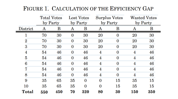
effectively used elsewhere. The following paragraph and Figure 1 chart (from reference 13 Stephanopoulos and McGhee) shows a hypothetical statewide vote described on p. 834 of that paper: “An example should illustrate
the intuitiveness of our measure. Take a state with 10 districts of 100 voters
each, in which Party A wins 55 percent of the statewide vote (that is, 550 votes).
Assume also that Party A wins 70 votes in districts 1–3, 54 votes in districts
4–8, and 35 votes in districts 9–10, and that the remaining votes are won by
Party B. Then Party A wastes 20 votes in districts 1–3, 4 votes in districts
4–8, and 35 votes in districts 9–10. Similarly, Party B wastes 30 votes in
districts 1– 3, 46 votes in districts 4–8, and 15 votes in districts 9–10. In
sum, Party A wastes 150 votes and Party B wastes 350 votes.14 The difference
between the parties’ wasted votes is 200, which when divided by 1,000 total
votes produces an efficiency gap of 20 percent. Algebraically, this means that
Party A wins 20 percent (or 2) more seats than it would have had the parties
wasted equal numbers of votes.”
Now looking simply at District 1,
the candidate for Party A received 70 votes to the 30 votes received by the
candidate for Party B. Since losing
votes are considered “wasted” votes (at least for purposes of winning the
current election, as opposed to something like perhaps giving a stronger than
expected showing of support or simply showing the number of people favoring the
candidate for Party B and opposing the candidate for Party A), it is clear that
the 30 votes for the candidate for Party B were wasted. However, it is not clear, and seems quite odd
or wrong, to say that the surplus votes for the candidate for Party A were 20,
instead of 39. The candidate for Party A
won by a 40 vote margin, not a 21 vote margin. A 40 vote winning
margin makes 39 of those votes unnecessary or surplus, not 20 of them
surplus. The 20 vote surplus seems to be
predicated on something like assuming that if those voters had not voted for
the candidate for Party A, they would have voted for the candidate for Party B,
but that would have tied the election in that district, not won it for the
candidate for Party A by the slimmest possible winning margin of 1 vote. If the assumption is going to be that voters
who don’t vote for the Party A candidate then flip to vote for the Party B
candidate, then the number of surplus voters in District 1 is 19, which would
make the vote totals be 51 – 49 in favor of the candidate for Party A. But if 39 of those voters for
the candidate for Party A did not vote at all, the candidate for Party A in
District 1 would have still won, by the margin of 1 vote, meaning that none of
the votes for him/her were wasted. Of
course, if 20 voters for the candidate of Party A flipped their votes to the
candidate of Party B instead, then the vote in District 1 would have been 50 –
50. So, even that way, 20 is not the
number of surplus votes for the candidate for Party A in district 1, but again
19 would be. In short, I see no reason why
the number of surplus votes is said to be exactly half the difference of the
number of votes between the two candidates in each district. And whatever that number represents, I don’t
see how it reflects wasted votes or inefficient votes. It seems that the number of surplus votes is simply
one fewer than the difference between the numbers of votes each candidate
received. In Districts 1 – 3, the
candidates for Party A each received 39 unnecessary votes, which presumably
count as ‘wasted’ votes, to win, and would have won 31 – 30 without them. In Districts 4 – 8, 7 of the winning votes
were unnecessary, and without them the votes would have been 47 – 46, still a
winning total and margin. Plus, the assumption that there
are straight Republican and straight Democratic voters sufficient
to vote in the candidate of the party with the greater number of members would
mean that it won’t matter who the candidates are or what their proposals are
for either party, which sometimes may be true, but is often not going to
be. In fact, part of the problem for
parties in general elections now is that extremists in both parties can control
the winners of the party primaries, but in doing so choose candidates less (or
even least) likely to appeal to the entire voting populace, and who may cause
enough voters in their own party to sit out the election (not vote at all) or
to vote for the opposing party’s candidate. As of this writing Republican Roy Moore in
Alabama is running again for a U.S. Senate seat he
lost in 2016 after credible allegations were made that he had behaved
inappropriately with underage females in the past. Many Republicans are concerned that he is
still popular enough among enough Republicans to win the primary and then get
beat again in the general election. Even
President Trump has called for Moore not to run in the primary for fear of
losing the predominantly Republican Alabama’s U.S. Senate seat to Democrats. One of the more interesting and astute
observations about the 2016 Presidential election was made by Trevor Noah just
after the Democratic and Republican nominating conventions were both over, when
he said both parties seem to have nominated the only candidate who could lose
to the other. And I don’t see, if voters may
choose crossover candidates, how one can accurately identify years prior to an election how many voters
there will be for one party or the other.
Suppose that in a previous election, the votes were 60/40 for the
candidate of Party A over the candidate for Party B. But suppose that in a subsequent election,
they vote 60/40 the other way. How do
you determine for redistricting purposes what party those voters will vote for? While it might be important for parties to
win the proportion of seats at least roughly commensurate with proportion of
votes they receive in an election, that latter number cannot be determined
ahead of time in order to design the districts to make it happen. It is dependent on how well the candidates or
their proposals will resonate with the voters.
In any given state, some candidates for a party will do better than
others. Beto
O’Rourke made the 2016 Senate election closer against Ted Cruz than many other
Democratic candidates may have done.
Whether O’Rourke would have done better or worse against a different
Republican is unknown. Gerrymandering
does often work, but it requires more stable, fixed voting patterns than may be
the case if politicians or parties are shrewd enough, as they are supposed to
be, to figure out how to attract voters (or progressive, principled, daring, or
as inept and out of touch enough to lose voters, as can happen) maybe even
sufficiently to flip districts in their or their opponent’s favor for a
particular election. When Lyndon Johnson
signed the civil right legislation, he correctly predicted that would cost
Democrats votes in the South for generations.
Eventually Dixiecrats just became the Republicans they at least halfway
had been for a long time. And even
though Barry Goldwater was soundly defeated in 1964, he helped launch a
conservative movement that eventually handed Ronald Reagan the Presidency. And Congressional majorities with Presidents
from the same party often lose seats in midterm elections. District voting is not necessarily stable or
predictable over the ten year period of districting
maps, even if gerrymandering can make some results more probable in the short
term. But moreover, there were 450
votes for the Party B candidate statewide overall and there were 550 overall
statewide votes for the Party A candidate.
If the 450 voters for the Party B candidate had been grouped evenly into
Districts 4 – 10, leaving none of them in Districts 1 – 3, they would have had 64
votes (64.2 mathematically, but you can’t have a fraction of a vote in
actuality) in each of 7 districts, thus winning 7 seats 64 - 36 instead of 2
seats, though they would have lost the seats in Districts 1 – 3 by votes of 100
- 0. The 550 votes for Party A’s
candidate (or 552 votes actually, because of the fraction aspect) would have
been divided into 36 for each of Districts 4 – 10, with 100 each in Districts 1
– 3. That means that the distribution
of voters in the hypothetical state is what determines the legislative
composition party-wise, not just the vote count. And it allows the party with 45% of the votes
to control 70% of the legislature. (If
you divided the 450 votes of Party B into 8 districts evenly, that 45% of the
electorate would win 8 districts or 80% of the legislature) by votes of 56 – 44, and lose two seats by votes of 100 – 0. But notice, if the voting
districts occurred naturally by geographic boundary lines of some sort or any
other ‘neutral, apolitical’ method of constructing them, it would not be unfair
in the way that it would seem to be unfair if Party B had designed the district
knowing that is how the vote would come out with that design. Whether Party A or Party B wins by a random, natural,
neutral or apolitical districting plan seems fair (though unfortunate for the
party that loses though it has a statewide majority of voters), in a way that
it seems totally unfair if the districts are designed by the party that then
wins the most seats because of that design. As Amy puts it (reference 1): Unintentional gerrymandering is
less well known than the deliberate variety, but it can also pose very serious
political problems. Even districting that is done with apolitical criteria will
likely produce many of the symptoms of gerrymandering – such as the creation of
many uncompetitive districts where one party dominates. The reason for this is
simple. Intentional gerrymandering is made possible by the geographic
concentrations of Republicans and Democrats – concentrations that can be split
and combined to provide advantages for a particular candidate
or party. Apolitical districting does not change that geographical fact. Thus many districts created by neutral criteria will
inevitably have concentrations of partisan voters that work in one party's
favor. Given that the same mathematical
outcomes can be both fair or unfair, depending on other factors, one can see
the Court’s reluctance to adopt a mathematical or statistical measure as an
indicator of either fairness or unfairness.
The fact that an unfair outcome will be lopsided doesn’t mean that a
lopsided outcome is unfair. In the
articles in the references section, there are numerous examples of unfair
districting boundaries, but that is shown by arguments that combine verbal
reasons along with numbers. Chief
Justice Roberts and the Court seem amenable to such arguments insofar as the
law allows them to be. But again, it is
important to remember that even if they accept that a districting plan is
totally unfair, that doesn’t mean they can rule it is unconstitutional or in
conflict with a higher order law, unless there is such a higher conflicting law
or constitutional provision they can point to. But also, since no matter how
the districts are constructed, they will pre-determine the outcome in favor of
one party or the other (or equally in the case of letting each side win 5
districts) if voters vote along strict party lines, it is not clear that one
outcome is more or less fair than any other. And which of the voters should be placed in
districts where they will be the minority party, essentially being sacrificed? It is difficult for me to tell
for sure, but the statisticians in these papers seem to hold or assume that the
fairest method is any one (or all the ones) that makes the outcome roughly
proportional to the proportion of party voters in the state. And I believe, but could be wrong, that besides
its being intuitive on its face, another argument is that the statistically most
probable outcomes of all possible designs will be the ones that yield the most
proportional representation and are thus the fairest because of that, and that
insofar as any design probabilistically causes a disproportionate outcome of
seats in the legislature compared with the proportion of votes the parties
received, it is to that extent an unfair or less than optimally fair design. Amy, who thinks the gerrymandering problem is
always going to exist with a single member plurality electoral system, and who
advocates scrapping it by adopting proportional representative elections, specifically
states: Indeed, the whole purpose of PR [proportional
representation] is to minimize wasted votes and ensure that the parties are represented in proportion to the votes they
receive. [Emphasis mine.] However, the U.S. Constitution
and methodologies and rules in the Senate and House of Representatives go to
great lengths, for good reason, to try to prevent tyranny of the majority (8 Garlikov),
with district representation in the House, combined with statewide representation
in the Senate as one of the mechanisms.
Insofar as Senators are elected by the proportional strength of the
parties in the states, you don’t want the House of Representatives elected in
the same way if they are to be an effective check and balance to the Senate. The federal government does not create law
based solely on simple majority vote of the Senate, House, and President. If it did, it would simply require a vote of
269 or more of the 536 of them combined.
And, as in many cases of
majority power, a mechanism that increases majority control over the minority
can be unfair and wrong, while the same mechanism if used to enhance relative
minority power and influence can be fair and right if it provides the minority
more of a voice and a ‘fighting chance’ at having their needs and interests
served. That is why in many cases what is considered to be ‘reverse discrimination’ is not as
invidious, unfair, or wrong as the discrimination it is meant to combat. Hence, gerrymandering that increases the
representational power of a minority may be right in a way that makes
gerrymandering to increase the power of the majority wrong. The morality of
strengthening an already strong advantage is opposite the morality of
strengthening the position of a severely unfairly disadvantaged group –
particularly as long as it does not harm the
advantaged group by hurting them, but instead lifts up the disadvantaged group. That is a principle behind the NBA and NFL draft
policies that given teams draft choices in reverse order of their previous
season finishes, so that the weaker teams have an opportunity to get stronger
players, though they are not thereby diminishing the strength of the previous
season’s stronger teams. The weaker
teams are just being given the opportunity to benefit more than the already
strong teams in order to make the leagues more competitive – and certainly far
more competitive than they would be if the already strong winning teams from
the previous season were able to draft first (without trading good players to a
weak team for their higher position in the draft). Party representation which is
proportional to population percentage is not necessarily meaningful or valuable
representation when it merely reinforces the power of the majority. To steal from Ephesians 5:25, it would indeed
be a blessing if majorities loved the minority as Christ loved the Church,
insofar as minorities have to be subject to the
majority. But that cannot be relied
upon. As John Stuart Mill wrote, “When
the well-being of society depends on the wisdom and benevolence of government,
it is at all times precarious.” Mechanisms are necessary to prevent power from
lapsing into tyranny. To borrow from Barry Goldwater, activism in defense of
fairness is not necessarily a vice. Reverse
discrimination, depending on how it is done, is not necessarily as unfair or
wrong as discrimination. And
gerrymandering to moderate the power of a majority to prevent tyranny if
necessary is not the same as gerrymandering to increase its power, especially
to dangerous levels. Unfortunately, any formal
mechanism, whether mathematical or verbal, is open to manipulation to thwart
its spirit while adhering to its letter (or numeric formulas), and that is
perhaps easier to get away with unrecognized with regard to
mathematical rules and formulas[1]. In Congress, gaming the system for personal
gain is a particular problem, due to the motivation
and ability of elected officials to combine in various sweetheart deals to
insure their own re-electability even at the expense of their state or the
country. As Amy and others point out,
some gerrymandering is not intended to insure victory of the contemporary
majority party but the continued re-election of incumbents of both sides. Constituent representation is a
mechanism intended to make government responsive to the needs, interests and
desires of the citizenry by allowing them to elect lawmakers knowledgeable of
and sympathetic to those needs, interests, and desires. Insofar as lawmakers are not members of your
circle, they are thought, often correctly, to be unaware or unconcerned --
ignorant of or apathetic to -- your community’s needs. That is perfectly reflected in Dave Barry’s
cynical description of the U.S. Senate at the time as being ‘100 old white male
millionaires looking out for you’. But a two party system doesn’t
tend to recognize or concern itself adequately to all the different interests
and needs citizens have, not only as individuals, but insofar as each citizen
is a member of many different overlapping or intersecting groups, some of which
or many of which may be minority groups of one sort or another, while others
are majority groups, whether based on gender, race, ethnicity, educational
level, region, political/philosophical views, health, wealth, family,
occupation, or any other factor that contributes to one’s opportunity to make contributions
to society and derive the benefits and burdens one receives from society,
whether in return for those contributions or not. For example, one might be male (majority) in
a legislature but be black or Muslim or poor, all likely minority
positions. So, what is necessary is to
have representatives who are sensitive to the needs and interests of everyone
as much as possible and motivated to meet them as well and as reasonably as all
available, and potentially available, resources can allow. This does not mean that membership in your
own group or district or subdistrict is either necessary or sufficient
to be understanding, motivated, or capable as a lawmaker. Those outside your group may be perceptive,
motivated, and able while those from your group may not be able, perceptive, or
caring. However, that cannot be relied
upon. What is needed are mechanisms to
protect minorities, mechanisms less subject to gaming or unfair manipulation. One way believed to at least try
to protect minorities is by requiring some legislative votes to have a
supermajority of, say 3/5 or 2/3 or even 3/4.
But I think a better way to try to make legislation palatable and/or
fair to minorities is instead to require that some reasonably fair percentage
of the minority concur with the overall majority vote because those members of
the minority think it fair (not because they are bought off or made a
sweetheart, logrolling, backscratching, favor trading, quid pro quo deal for
their vote, etc.). For example, suppose Party
A comprises 76% of the legislature and will vote along party lines. They can then pass any supermajority
legislation without the support of the minority, effectively disenfranchising
the minority effected by that issue, whether the issue is one of race, gender,
age, wealth, religion, ethnicity, place of birth, liberal versus conservative, weather
conditions, geographical needs, urban versus rural versus suburban, employee versus
employers, etc. But if they needed a simple majority of the total
votes to include some reasonable proportion of the minority or those most
effected or disadvantaged by the legislation, in order to pass it, that could
be fairer. It would also more than
likely lead to accommodation by the majority for the needs and interests of the
minority in designing legislation, whereby accommodation is not about
compromise (which may please no one) but about serving common interests to the
maximum extent possible. For example, suppose some tax is
proposed on people with more than 10 million dollars in order to fund some
specific project. Since, as of this
writing, there are far fewer people with 10 million dollars than there are
people with less than 10 million dollars, whatever percentage of overall votes
or supports for votes required to pass the measure should have to include some
percentage of votes or support, say 30% maybe, of people with more than 10 million
dollars. Normally that would require
designing the project in a way that multimillionaires would feel is at least
worthwhile and reasonable enough to support.
Setting the reasonable percentages of the necessary minority concurrence
for different issues will require reasoning through the process in some way and
may perhaps need to be in some proportion to the seriousness or hardship of the
effects on the minority or disadvantaged group involved. But what would determine whether
this system is really fair or not. Assuming it captures some sense of fairness,
what percentage of minority votes would you need for it to be fair? And what if it affects different minorities
in different ways? Do certain
percentages of each of their different memberships have to vote for the
bill? What would determine whether you
have got the percentages or even the method right to make it fair? Would the minority party position have to win
50% of the time or near it for the method to be fair? That doesn’t seem to me to necessarily
reflect the kind of fairness at issue.
And it may be part of why a mathematical way of calculating fairness,
particularly an abstruse one, finds Chief Justice Roberts reasonably unwilling
to accept one as the test or as a significant measure for fairness in
redistricting for elections. References: 1.
Amy, Douglas J.
How Proportional Representation Would Finally Solve Our Redistricting
and Gerrymandering Problems. Fair Vote. 2. Brams, Steven J. The Hill. Making partisan gerrymandering fair https://thehill.com/opinion/campaign/405426-making-partisan-gerrymandering-fair 3. BRIEF OF HEATHER K. GERKEN, JONATHAN N. KATZ, GARY KING, LARRY J. SABATO, AND SAMUEL S.-H. WANG AS AMICI CURIAE IN SUPPORT OF APPELLEES https://www.brennancenter.org/sites/default/files/legal-work/Gill_AmicusBrief_HeatherK.GerkenEtAl_InSupportofAppellees.pdf 4. Garlikov, Rick. Examples of a Common Kind of Fallacy in the Social Sciences. http://www.garlikov.com/philosophy/SocialScienceFallacyExample.html 5. Garlikov, Rick. The Electoral College, Fairness, and Sports http://www.garlikov.com/philosophy/ElectoralCollegeAndSports.html 6. Garlikov, Rick. The Left-Right Divide in America and the Problem of Voting for People Rather Than Ideas http://www.garlikov.com/philosophy/LeftRightDivideInAmerica.html 7. Garlikov, Rick. The Logic and Fairness/Unfairness of Gerrymandering http://www.garlikov.com/philosophy/Gerrymandering.html 8. Garlikov, Rick. The Need for Formal and Informal Mechanisms to Prevent "Tyranny of the Majority" in Any Democratic Government http://www.garlikov.com/philosophy/majorityrule.htm 9. Greenblatt, Alan November, 2011, Governing The States and Localities https://www.governing.com/topics/politics/can-redistricting-ever-be-fair.html 10. Grofman, Bernard and King, Gary. The Future of Partisan Symmetry as a Judicial Test for Partisan Gerrymandering after LULAC v. Perry. ELECTION LAW JOURNAL Volume 6, Number 1, 2007 © Mary Ann Liebert, Inc. DOI: 10.1089/elj.2006.0000 https://gking.harvard.edu/files/jp.pdf 11. Liptak, Adam. The New York Times. January 15, 2018. A Case for Math, Not ‘Gobbledygook,’ in Judging Partisan Voting Maps. https://www.nytimes.com/2018/01/15/us/politics/gerrymandering-math.html 12. McGhee, Eric. SCOTUSblog. “Symposium: The efficiency gap is a measure, not a test” August 11, 2017. https://www.scotusblog.com/2017/08/symposium-efficiency-gap-measure-not-test/ 13. Nicholas O. Stephanopoulos, Nicholas O. and McGhee, Eric M. The University of Chicago Law Review. 2015. Partisan Gerrymandering and the Efficiency Gap http://uchicagolawjournalsmshaytiubv.devcloud.acquia-sites.com/sites/lawreview.uchicago.edu/files/04%20Stephanopoulos_McGhee_ART.pdf 14. Princeton Gerrymandering Project. http://gerrymander.princeton.edu/info/ 15. Princeton Gerrymandering Project. http://gerrymander.princeton.edu/ 16. Wang, Sam and Remlinger, Brian. How to spot an unconstitutionally partisan gerrymander, explained. Vox. Jan 17, 2018 https://www.vox.com/the-big-idea/2018/1/17/16898378/judges-identify-partisan-gerrymandering-north-carolina-supreme-court 17. Wang, Sam. New York Times. Let math save our democracy. December 5, 2015. https://www.nytimes.com/2015/12/06/opinion/sunday/let-math-save-our-democracy.html 18. Wang, Sam. New York Times. July 13, 2019. If the Supreme Court Won’t Prevent Gerrymandering, Who Will? A progressive take on states’ rights can come to the rescue. https://www.nytimes.com/2019/07/13/opinion/sunday/partisan-gerrymandering.html 19. Wang, Sam. Gerrymandering, or Geography? Computer-based techniques can prove that partisan advantage isn’t an accident. The Atlantic March 26, 2019 https://www.theatlantic.com/ideas/archive/2019/03/how-courts-can-objectively-measure-gerrymandering/585574/ 20. Wang, Samuel S.-H. Three Tests for Practical Evaluation of Partisan Gerrymandering Stanford Law Review. Volume 68. June, 2016. http://www.stanfordlawreview.org/wp-content/uploads/sites/3/2016/06/3_-_Wang_-_Stan._L._Rev.pdf 21. Wang, Samuel S.-H. Three Practical Tests for Gerrymandering: Application to Maryland and Wisconsin ELECTION LAW JOURNAL Volume 15, Number 4, 2016 © Mary Ann Liebert, Inc. DOI: 10.1089/elj.2016.0387 https://web.math.princeton.edu/~sswang/wang16_ElectionLawJournal_gerrymandering-MD-WI_.pdf [1] I was going to illustrate this point by reference to handicap in golf as I had learned it as a young caddy, but it turned out when I researched it, that what I had learned as a simple calculation either was erroneous or has since been replaced by an extremely complex, elaborate mechanism that illustrates the point I want to make even better. What I had been told constituted a golf handicap was “80% of the difference between par for the course and the average of your last 10 scores.” So if you averaged shooting 81 on a par 71 course, your handicap would be 8, meaning that you get a stroke off your score for each of the 8 most difficult holes on the course when you play golf for friendly competition that allows handicap to be used. The scorecard ranks the holes in order of degree of difficulty, so you know which holes you get strokes on. The point of handicap is to allow competition to be more even and not predetermine the winner despite one player’s having more, even far more, skill than another. And it means that if one player on average has a legitimate (not ‘sandbagging’; i.e., not purposefully higher than normal in order to raise his/her handicap artificially) score 10 shots better on the course than another, he has to concede a stroke on each of eight holes to the weaker player. And the weaker player’s handicap is also meant to be based on an honest set of scores, not sandbagged ones. Notice that still gives the stronger player a 20% advantage. I don’t know how the 80% figure was chosen instead of 100%, and it seems on the surface of it that if two players differ in their ability by 10 strokes a round on that course that the way to “even up” the competition between them would be for the stronger player to have to concede a stroke on each of ten holes. And whether the strokes should be on the relatively most difficult holes, or chosen in some other way, also seems perhaps arbitrary. But modern golf computes handicap in a far more complex way that takes into account degree of difficulty of the course being played versus other courses, and it does so involving a formula that considers the different degrees of difficulty for really good players (called ‘scratch’ players -- those likely to shoot par or close) versus those not as good and likely to shoot closer to a stroke over par per hole (bogey golfers). However, for purposes of the formulas used to compute relative degrees of difficulty, scratch and bogey players are defined not by their scores alone but by a particular range of scores and objective abilities about how far they can hit a ball and how many shots it takes them to reach the green on a given hole, particularly depending on obstacles on the hole. The official definition of a bogey golfer is "A player with a USGA Handicap Index of 17.5 to 22.4 strokes for men and 21.5 to 26.4 for women. Under normal situations the male bogey golfer can hit his tee shot 200 yards and can reach a 370-yard hole in two shots. Likewise, the female bogey golfer can hit her tee shot 150 yards and can reach a 280-yard hole in two shots. Players who have a Handicap Index between the parameters above but are unusually long or short off the tee are not considered to be a bogey golfer for course rating purposes."(https://www.liveabout.com/bogey-golfer-definition-1560779) And the following is how to compute your handicap for a given course (from http://golfsoftware.com/hsd/golf-handicap-formula.html, with editing): Step 1: Convert Original Gross Scores to
Adjusted Gross Scores To arrive at an Adjusted Gross Score, you use the USGA's
Equitable Stroke Control (ESC). ESC is used to downwardly adjust individual
hole scores for handicapping purposes … ESC imposes a maximum number of strokes
that can be entered for any given hole. This
maximum is based on the golfer's Course Handicap and is obtained from [a] table Step 2: Calculate Handicap Differentials for
Each Score using the following formula: Handicap Differential =
(Adjusted Gross Score - Course Rating) X 113 ÷ Slope Rating (The Course Rating is what the USGA deems a scratch golfer
would score on a course under normal playing conditions. A Slope Rating of 113
is for a course of standard difficulty according to the USGA.) [It is the slope
of the line connecting a scratch golfer’s score with a bogey golfer’s score,
where scratch and bogey golfers are defined in a technical way that doesn’t
mean scratch golfers shoot par or that bogey golfers shoot 18 over par.] Round the Handicap
Differential to the nearest tenth (i.e., 17.25=17.3, 11.34=11.3, etc.). Step 3: Select Best, or Lowest, Handicap
Differentials Step 4: Calculate the Average of the Lowest
Handicap Differentials Step 5: Multiply Average of Handicap
Differentials by 0.96 or 96% [This gives a slight edge to better
golfers for being better and is thought to be fairer to them.] Step 6: Truncate, or Delete, Numbers to the
Right of Tenths This gives you your “Handicap Index” Step 7: Calculate Course Handicap The final step is to calculate a Course Handicap. A Course
Handicap is the number of strokes a player receives on each particular course.
Determine a course handicap by multiplying the Handicap Index by the Slope
Rating (from the course and tee you choose) and dividing by 113 (standard
difficulty rating). Round the result to the nearest whole number. Course Handicap = Index x (Slope Rating of Tee
on Course / 113) Suppose you work with all this until you can understand
what it means and how to use it, so that you see it computes 96% of how much
above par you usually are when you play at your best on the courses you have
played, relative to an average course, and then it applies that to any course
you might play, based on its relative degree of difficulty to the average
course, as determined by specified procedures. My question is “How would you test all this” in order to
determine whether it truly makes a match between two golfers – especially one
much better than another – even and fair in the sense of not being able to tell
ahead of time who will win or perhaps who will even more likely win? Would you have to see how it works out with a
great many matches? Has anyone done
that? How close does it have to be to
50/50 between better and worse golfers in order to be fair in that sense of
fairness? And notice, it doesn’t mean
that if the weaker golfer wins, even many times, that he is the better golfer;
it just means s/he won when given this particular handicap computed in this
particular way.
|